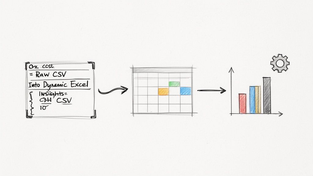
Building a proper report in Excel is all about a simple transformation: taking a mountain of raw data, like a basic CSV file, and turning it into a clean, structured table. From there, you can summarize everything with Pivot Tables and bring the story to life with charts. The end goal is a clear, reusable dashboard that makes sense of scattered updates and gives you real, actionable insights.
From Data Chaos to Reporting Clarity
Let's be honest, most of us are drowning in digital noise. Trying to track progress effectively often feels like an impossible task, leading to wasted time and frustrating status meetings. This guide is designed to be your way out of that chaos. I'll walk you through how to take a simple data export, say, from a work-logging tool like WeekBlast, and build a powerful, automated report right inside Excel.
This whole process is about moving from messy, raw data to a report that actually tells you something useful.
As you can see, the secret isn't just having the data; it's structuring it to tell a clear story. Forget complicated project trackers. We're focused on a practical approach: turning your team's day-to-day updates into a visual narrative of progress that helps you make decisions, all without the soul-crushing manual work.
Why Structured Reporting Matters
In today's workplace, the need for clear, concise reporting has never been greater. We're all fighting an uphill battle against a constant stream of information and interruptions that shatter our focus.
Consider this: the average office worker gets a mind-boggling 117 emails every single day. On top of that, they're interrupted roughly every two minutes, which adds up to 275 interruptions daily. With that much context-switching, keeping a clear picture of project progress is next to impossible without a solid system in place. If you're curious, you can learn more about these workplace statistics to see just how deep the problem runs.
A well-built Excel report cuts right through that noise and becomes your single source of truth. It works by:
- Centralizing Updates: It pulls all those scattered work logs and updates into one coherent view.
- Providing Quick Insights: Dashboards give you an immediate, at-a-glance understanding of where things stand.
- Reducing Manual Effort: Once you set up the automation, you spend less time compiling data and more time actually analyzing it.
By investing a little time upfront to build a proper report structure, you're essentially buying back hours of your future self's time. You reclaim the hours previously lost to manual data wrangling and repetitive status updates. This is how you shift from relying on memory or scattered notes to making truly data-driven decisions.
Getting Your Raw Data Ready for Analysis
Before you can even think about building an insightful report, you have to start with clean, reliable data. I can't stress this enough. So many people rush this part, only to get frustrated later when their charts are wrong or their formulas break. The truth is, your final report is only ever as good as the data you start with.
This whole process kicks off the moment you import your raw data. Maybe it’s a CSV file you've just exported from a tool like WeekBlast. Raw exports are almost never perfect. They're usually littered with little issues that can trip you up, like extra spaces, wonky date formats, or numbers that Excel thinks are text.
Luckily, Excel has some fantastic built-in tools to handle exactly these kinds of messes.
Cleaning and Structuring Your Dataset
Your first job is to play detective and hunt down all the subtle errors that can wreck your report. A classic example? An extra space at the end of a word. It seems harmless, but it can make Excel see two identical entries as completely different things, which completely skews your counts and sums.
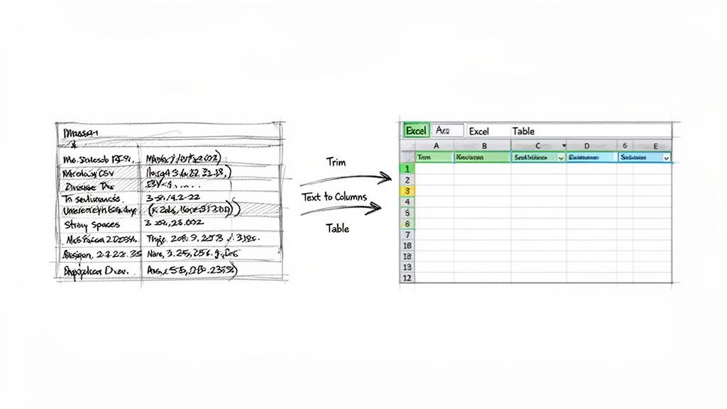
This is where a couple of simple tools become your absolute best friends: the TRIM function and the Text to Columns feature.
- TRIM Function: This little gem of a formula (
=TRIM(A1)) zaps all the extra spaces from the start and end of your text. It's a lifesaver for cleaning up things like client names, project titles, or categories that have inconsistent spacing. - Text to Columns: This is a powerhouse for splitting data from one column into several. Let's say you have a single column with both a date and a time in it. With Text to Columns, you can easily break them apart into two separate, usable fields.
These small cleanup steps aren't just about being neat. They're about locking in the integrity of your data before you get to the fun stuff.
Key Takeaway: The single most important thing you can do at this stage is to convert your clean data range into a proper Excel Table. This isn't just about adding some fancy stripes to your spreadsheet; it's a fundamental structural change that makes everything that follows easier and more accurate.
To get you started, here's a quick rundown of the most common data cleaning tasks you'll likely encounter.
Common Data Cleaning Tasks in Excel
| Problem | Excel Tool/Function | What It Does |
|---|---|---|
| Extra leading/trailing spaces | TRIM() |
Removes unnecessary spaces from the beginning or end of text. |
| Inconsistent text case | UPPER(), LOWER(), PROPER() |
Converts text to all uppercase, all lowercase, or title case. |
| Numbers stored as text | VALUE() or "Convert to Number" |
Changes text that looks like numbers into actual numeric values. |
| Data combined in one cell | Text to Columns | Splits a single column of text into multiple columns based on a delimiter. |
| Blank rows or cells | Go To Special > Blanks | Quickly finds and allows you to delete all empty cells or rows. |
| Duplicate records | Remove Duplicates | Identifies and deletes entire rows that are exact copies. |
Familiarizing yourself with these tools will save you countless hours and prevent a lot of headaches down the road.
The Power of a Proper Excel Table
Turning your data into an official Table (just select your data and hit Ctrl + T) is a non-negotiable step in my book. It’s what transforms your report in excel from a static, fragile thing into something dynamic and robust.
Once your data is inside a Table, you get some amazing benefits right away.
Any formula referencing the Table automatically expands as you add new data, which means you never have to manually adjust your ranges again. That feature alone is a massive time-saver and a huge guard against errors.
Plus, Tables come with built-in sorting and filtering controls right in the header row, making it incredibly easy to inspect and work with your data. This simple conversion creates the solid foundation you need for all the powerful analysis you're about to do with Pivot Tables and charts.
Turning Raw Numbers into Real Answers with Pivot Tables and Charts
Alright, your data is now clean, organized, and sitting nicely in a proper Excel Table. This is where the fun really begins. We’re about to move from a flat list of entries into the world of dynamic analysis, transforming raw numbers into meaningful insights. We'll be using two of Excel's most powerful tools for this: Pivot Tables to summarize the data and Pivot Charts to tell its story visually.
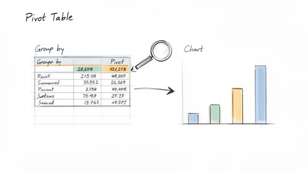
Think of a Pivot Table as a flexible analysis engine. It takes all your neatly structured data and lets you slice, dice, and group it in countless ways, all without writing a single formula. It's the perfect way to graduate from an endless scroll of individual tasks to a high-level summary of your team's efforts.
From Raw Data to Actionable Summaries
Getting started with your first Pivot Table is surprisingly straightforward. Just click any cell inside your Excel Table, head to the Insert tab, and select PivotTable. Excel is smart enough to detect your entire table as the source. I'd recommend placing the Pivot Table on a new worksheet to keep your workbook tidy.
Once you do that, the PivotTable Fields pane will pop up on the right. This is your control panel. You'll see a list of all your column headers (like "Team Member," "Project," or "Hours Spent") at the top and four boxes at the bottom: Rows, Columns, Values, and Filters.
I see a lot of people get overwhelmed by the options here. The trick is to ignore the complexity and start with one simple question. For instance: "How many hours did each person log for Project Phoenix?" You can answer this in seconds by dragging "Team Member" to the Rows box, "Hours Spent" to the Values box, and then dropping "Project" into the Filters box to select 'Project Phoenix'. Just like that, you have your answer.
This drag-and-drop functionality is the real magic of Pivot Tables. You can rearrange fields on the fly to explore different questions. What happens if you swap "Team Member" and "Project" in the Rows box? You instantly get a new report showing a breakdown of hours per project instead of per person.
Asking the Right Questions with Your Data
The true value of a Pivot Table is its ability to answer business questions that would otherwise require tedious manual filtering and calculations. With a few clicks, you can uncover insights buried in your data.
Using a typical work log export from a tool like WeekBlast, here are a few questions you could answer almost instantly:
- Who completed the most tasks last month? Drag "Team Member" to Rows and a count of "Task ID" to Values.
- Which project is eating up the most time? Put "Project Name" in Rows and the sum of "Hours Spent" in Values.
- What's the average time we're spending on different types of tasks? Add "Task Category" to Rows and the average of "Hours Spent" to Values.
This dynamic approach helps you spot trends you’d almost certainly miss otherwise. You might discover that one person is consistently tackling the most difficult tasks or that a particular project is consuming far more resources than anyone realized.
Visualizing Your Findings with Pivot Charts
Once you've arranged your Pivot Table to show a useful summary, the next step is to visualize it. A Pivot Chart is linked directly to your Pivot Table, which is a huge time-saver. Any change you make to the table, whether it's adding a filter or refreshing the underlying data, is automatically reflected in the chart.
Creating one is simple. Click anywhere inside your Pivot Table, find the PivotTable Analyze tab that appears in the ribbon, and click PivotChart.
Choosing the right chart type is critical. The goal is to tell a clear story, so don't just default to the first option you see. Think about the message you want to convey.
- Bar/Column Charts: These are your go-to for comparing totals across categories. Think hours per project or tasks completed by each team member.
- Line Charts: Perfect for showing trends over time. Use these to track things like team productivity week-over-week or the number of bugs resolved each month.
- Stacked Bar Charts: Great for showing how different parts contribute to a whole. You could use one to show a project's total hours broken down by task type (e.g., Design, Development, Testing).
By combining a powerful summary with a clear visual, you transform a simple spreadsheet into an interactive report that communicates progress and shines a light on what needs attention.
Building a Reusable Excel Report Template
A one-off analysis is useful, but a reusable report template? That's a total game-changer. You’ve already done the heavy lifting by summarizing your data with Pivot Tables and creating charts. Now it's time to bring it all together into a professional, interactive dashboard. This is how you turn a static spreadsheet into a dynamic tool that empowers your team to explore the data for themselves.
The whole point is to create a single, clean sheet where anyone can get a high-level overview at a glance, then dive into the specifics that matter most to them. This is the heart of an effective report in excel; it serves both the big-picture viewers and the detail-oriented analysts.
Arranging your dashboard is a mix of art and science. I always tell people to think like a newspaper editor: put the most critical information, your headline KPIs and summary charts, in the top-left corner. That's where the eye naturally lands first. From there, you can let the supporting details and more granular charts flow down and to the right.
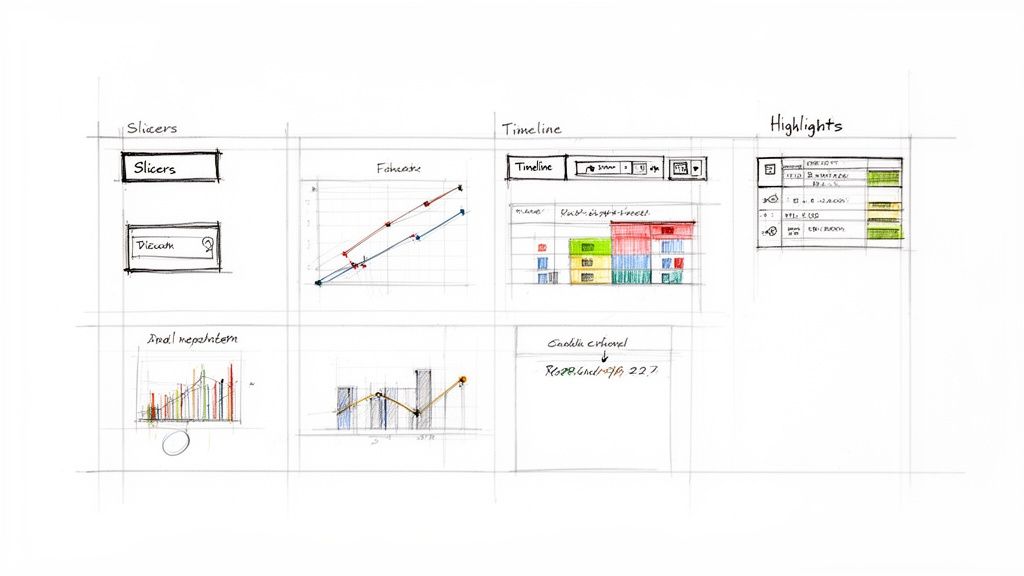
Making Your Report Interactive with Slicers
The real magic of a dashboard lies in its interactivity. You want your colleagues to be able to answer their own questions without having to become Excel gurus. Your best friends for this are Slicers and Timelines.
Slicers are basically just fancy, user-friendly buttons that filter your Pivot Tables and charts. Instead of making someone fiddle with those clunky filter dropdowns, you can give them clean, obvious options to click.
Adding one is simple:
- Click anywhere inside one of your Pivot Tables.
- Head to the PivotTable Analyze tab in the ribbon.
- Select Insert Slicer and pick the fields you want to filter by, things like "Team Member," "Project," or "Task Category" are perfect for this.
A Timeline is a special kind of slicer built just for dates. It provides a slick visual slider that lets users filter the report by day, month, quarter, or year. It’s absolutely brilliant for spotting productivity trends over different timeframes.
Here's a pro-tip that many people miss: you can connect a single slicer to multiple Pivot Tables. Just right-click the slicer, choose "Report Connections," and tick the boxes for every Pivot Table you want it to control. With that one move, a single click can filter your entire dashboard simultaneously.
Highlighting Key Metrics Automatically
With your dashboard now interactive, the final layer is adding visual cues that automatically draw attention to the most important numbers. This is where Conditional Formatting truly shines. It lets you program a cell to change its appearance, like its background color or font style, based on the value it contains.
This technique is what elevates your report from just being informational to being genuinely actionable. For this to work well, you need good data to begin with; using a daily work log template is a great way to ensure you're collecting the right info from the start.
Here are a few practical ways I use it all the time:
- Spotting outliers: I'll apply a color scale to a column of hours worked. The cells with the highest values automatically get a darker shade, instantly showing which projects are eating up the most time.
- Flagging performance issues: You can set a simple rule to turn a cell red if, say, the number of tasks completed in a week drops below your target.
- Visualizing progress: "Data Bars" are fantastic for this. They create small bar charts right inside the cells, making it incredibly easy to compare values in a list without needing a separate, full-sized chart.
By combining a smart layout, interactive slicers, and clever conditional formatting, you’ve built something far more valuable than a simple analysis. You’ve created a durable, reusable template that will save you and your team hours of work every single week.
Automating Your Reporting with Power Query
What if you could update your entire report with a single click? I'm serious. Instead of dreading that manual data-cleaning slog week after week, you can build a system that does all the heavy lifting for you. This is where the real magic of automation comes in, and Excel's best-kept secret for it is a tool called Power Query.
Think of Power Query as a macro recorder for your data prep. It watches every cleaning and shaping step you take, removing extra spaces, splitting columns, changing data types, and records it. Once you build this repeatable process (called a query), you can run it on any new data file with a simple refresh. The time savings are incredible.
This completely changes how you create a report in excel. It shifts your energy away from tedious, repetitive tasks and lets you focus on high-value analysis, which is where your expertise truly shines.
Your First Automation Workflow
Getting started with Power Query is a lot more approachable than it sounds. You don't need to be a coding wizard to build a robust automation sequence. The interface is visual and records your actions as you click through familiar menus and options.
Your first move is to connect to your data source. This is typically the CSV file you exported from your work-logging tool, but it could also be an entire folder of files.
Here’s how you get the ball rolling:
- Head to the Data tab in the Excel ribbon.
- In the Get & Transform Data group, find and click on From Text/CSV.
- Browse to your data file, select it, and click Import.
This launches the Power Query Editor, a separate window where all the transformation happens. This is your new command center. From here, you can apply all the cleaning steps we covered earlier (like trimming text or changing formats) just by clicking buttons in the ribbon.
Every change you make gets added as a step in the "Applied Steps" list on the right side of the screen. This creates a repeatable recipe that Excel will follow flawlessly every single time you refresh the data, guaranteeing consistency and wiping out human error.
From Manual Drudgery to a Single Click
Once you've set up all your cleaning and transformation steps in the Power Query Editor, you just click "Close & Load". Power Query runs your entire sequence and drops the perfectly clean data into a new worksheet, already formatted as a proper Excel Table. This table is now the rock-solid foundation for your Pivot Tables and charts.
The next time you get a new weekly data export, the process becomes almost laughably simple:
- Save the new file in the same location (you can even just replace the old one).
- Open your master Excel report.
- Go to the Data tab and click Refresh All.
That’s it. Power Query instantly reruns your entire cleaning sequence on the new data, and all your connected Pivot Tables and charts update automatically. A reporting process that used to take an hour of painstaking manual work is now done in seconds. If you're looking for more ways to cut down on manual work, check out our guide on the core principles of automating data entry.
Sharing and Presenting Your Excel Report
You've done the hard work of wrangling the data and building a powerful report. But a great report sitting on your hard drive doesn't help anyone. The real magic happens when you get it into the right hands so people can understand it and make decisions.
Before you hit 'send,' it's smart to do a quick clean-up. Think of it as staging a house before a showing. I always hide my raw data tabs, get rid of any scratchpad sheets I used for calculations, and reset all the slicers to a sensible default view. This way, whoever opens it sees a polished, ready-to-use dashboard, not my messy workbench.
Getting Your File Ready to Go
The last thing you want is for someone to accidentally delete a formula and break the entire report. A simple but effective trick is to protect the worksheet.
You can lock down all the cells containing your charts and formulas while leaving the slicers and filters unlocked. This gives your colleagues the freedom to play with the data and dig into their specific areas of interest without any risk of messing up your handiwork.
Also, consider the format. Sending the live .xlsx file is great for interactivity, but sometimes you need a static snapshot. For a board meeting or a formal weekly summary, a PDF is often the better call. It’s clean, professional, and prevents any "oops" moments.
I've learned this the hard way: match the format to the audience. Your manager who just needs the bottom-line numbers will thank you for a simple PDF, while your teammate who needs to drill down into the details will want the interactive Excel file.
Picking the Best Way to Share
How you send the report can be just as important as the data inside it. Emailing an attachment is the old-school way, and it works, but we have better options now.
- Export to PDF: This is my go-to for a final, "official" version. It’s a clean snapshot that looks good on any device and locks in your findings. Perfect for archiving or attaching to a formal update.
- Use OneDrive or SharePoint: When you need the team to have live access, sharing the file on a cloud platform like OneDrive or SharePoint is the way to go. You get version control and can set permissions for who can view versus who can edit.
- Protect the Workbook: If you're dealing with sensitive information, add a password. You can set one password to open the file and another to modify it, which gives you an extra layer of control.
At the end of the day, your job isn't just to present data; it's to tell a story. Don't just send the file; walk your team through it. Point out the key insights, explain what the numbers mean, and connect them to your project goals. For more strategies on crafting compelling updates, check out our guide on effective work reporting. Your goal is to turn that spreadsheet into a conversation that drives action.
Stop losing track of your progress. WeekBlast turns scattered updates into a clear, searchable log of your work, making reports and reviews effortless. Never forget the work you did.


